Dijkstra's algorithm can be used to calculate the shortest paths from a start node to each node of the graph. The algorithm can be applied to both directed and undirected graphs. However, it is important that the edge weights must not be negative.
Application
A classical application area for Dijkstra's algorithm is route planning. Here, nodes model intersections. That is, places where you can decide on a direction. Edges model the roads between the intersections. The edge weights can be the duration needed to cover the distance between 2 intersections. Depending on the application, it may also be useful to include the distance traveled or the fuel consumption.
How it works
Pseudocode:
Input:
Dijkstra's algorithm is given a set of nodes V, a set of edges E and a starting node start∈V.
Important values and quantities:
A set of nodes Q⊆V is needed, which contains all nodes to which potentially no shortest path has been found yet.
Each node v∈V is assigned a distance value distance[v]. This is the length of the shortest path from the start node start to the node v, on which at most v may still be contained in Q. If such a path does not exist, distance[v]=∞ applies.
Furthermore, for each node v∈V there is a predecessor predecessor[v]. If a path is found which, apart from possibly v itself, contains only nodes that have already been removed from Q, then predecessor[v] is the direct predecessor of v on that path. Otherwise, predecessor[v]=null. With the help of these predecessor values, the path from v to start can be traced back.
Goal:
After running the algorithm, for each v∈V, if there is a path from start to v, distance[v] contains the length of the shortest path from start to v and predecessor[v] is the direct predecessor node on the path. If there is no such path, distance[v]=∞ and predecessor[v]=null remain.
Initialization phase:
The start node is assigned the distance value 0, all others get ∞ as distance value.
All nodes are assigned null as predecessor node.
All nodes are inserted into Q.
Loop:
In each loop cycle, the element u∈Q with the lowest distance value distance[u] is extracted from Q first. Then, for each direct successor node v∈Q of u, we examine whether the path from start to v via u is shorter than the shortest path found so far. If this is the case, the distance value of v is set to the length of the path from start to v via u (distance[v] := distance[u] + weight(u, v)) and u becomes the new predecessor node of v. The new shortest path found so far from start to v thus runs over u with u as the direct predecessor of v.
This is done until Q is empty.
Small example:
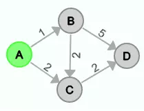
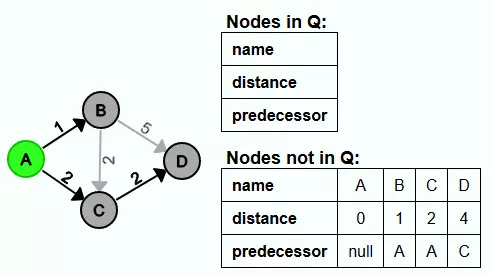
Given the following small example graph with A as the start node.
Initialization:
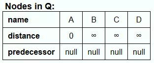
First, all nodes are initialized as described above and inserted into Q.
Iteration 1:
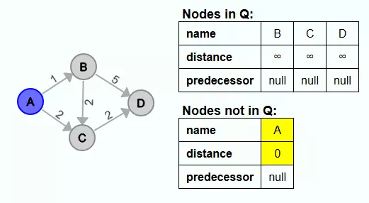
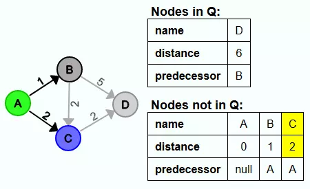
In the first iteration, the starting node A is the node with the smallest distance value. It is the only node whose distance value is not ∞.
Since no path has been found for B and C and the distance value is therefore ∞, A becomes the new predecessor node of B and C and the distance values are adjusted.
Iteration 2:
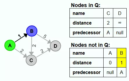
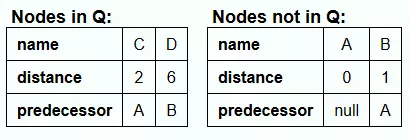
Now B is the node with the smallest distance value in Q. So it is deleted from Q.
No path has been found for D so far. So B becomes the new predecessor node of D and the distance value of D is adjusted.
The path from A to C via B is longer than the shortest path so far. So A remains the predecessor of C.
Iteration 3:
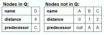
The distance value of C is smaller than that of D. So this time C is removed from Q.
The path from A to D via C has a length of 4 and this is shorter than the shortest path found so far with a length of 6. Thus, the path via C becomes the new shortest path. So the distance value of D is set to the length of the path from A to C + the edge weight of C to D and C will be the new predecessor.
Iteration 4:
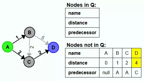
D is the only element in Q and thus also the one with the shortest distance value. Therefore D is now removed from Q.
Q is now empty. Each node is now assigned the length of the shortest path from A to the node, and the paths can be reconstructed via the predecessors.
Implementation notes
Priority queue:
For efficiency reasons, a so-called priority queue is often used for Q.
Adjacency list:
Graphs are often stored as adjacency lists. For this purpose, a list of successor nodes (or, in the case of undirected graphs, neighbor nodes) and the edge weights are stored for each node. The Dijkstra algorithm can be applied well to adjacency lists.
Modifications
fixed target:
In practice, one often does not want to determine the shortest paths to all nodes, but only to a very specific one. When this is reached, the algorithm can be canceled.
multiple start nodes:
There are use cases where more than one start node makes sense. For example, a company might want to deliver a product that is in stock at multiple company locations to a customer. All of these locations could be possible start nodes. In this case, one can modify Dijkstra's algorithm to pass it a set of start nodes. In the initialization phase, each of the nodes in the starting node set must then be assigned the distance value 0.
Cancel when only unreachable nodes are left in Q:
If the node in Q with the smallest distance value has the distance value ∞, it means, that the node cannot be reached from the start node. Since in Q there can no longer be a node with a lower distance value, all other nodes in Q are also no longer reachable from the start node. Thus, the Dijkstra algorithm can be canceled.
not all nodes in Q
One does not have to insert all nodes from the beginning in Q. One can also insert only the start node and if from the smallest element just considered an edge leads to a node that is neither in Q nor has been in it before, it is inserted into Q. This means that in practice there are often fewer nodes in Q at the same time, which means that the data structure used can often be managed more efficiently.
